Program Options
Important
This documentation is not meant to go over all the physics/astronomy or background knowledge required to fully understand what the various programs are doing.
IRAF Reduction
Note
The pipeline for this program is set up only for use at BSUO. This will be updated in the future.
Making heavy use of Astropy’s ccdproc and Photutils, this program provides an automatic data reduction process using Bias, Dark, and Flat frames to reduce science images.
The GUI panel accepts the following inputs:
Raw Images Path — folder containing the raw, unreduced FITS images
Calibrated Images Path — folder where reduced images will be saved
Location — telescope site identifier (e.g. BSUO, CTIO)
Use Dark Frames — checkbox to include or skip dark frame subtraction
Overscan Region — format
[columns, rows], e.g.[2073:2115, :]Trim Region — format
[columns, rows], e.g.[20:2060, 12:2057]
A Open Bias Image button is provided to plot row 1000 of a selected bias frame, helping the user identify the overscan and trim regions before running the reduction.
Note
For ccdproc, if the same rows are entered for both the overscan and trim region,
ccdproc will error out. The recommendation is to use all rows (:) for the
overscan region and specify exact rows only for the trim region.
Default Values
The reduction uses the following default camera parameters which can be overridden in the GUI:
Gain — 1.43 e⁻/ADU
Read Noise — 10.83 e⁻
Memory Limit — 450 MB (
450e6)
Reduction Functions
The main reduction stages are bias, dark, flat, and science. Each calls
a shared reduction function for the actual image processing:
Bias
The bias reduction subtracts the overscan and trims each raw bias frame, then combines them into a master bias using sigma clipping:
def bias(files, calibrated_data, overscan_region, trim_region, log, cancel_event):
    """
    Calibrates bias images and creates a master bias.

    :param files: Image file collection
    :param calibrated_data: Path to save calibrated images
    :param overscan_region: String for the overscan region of the CCD
    :param trim_region: String for the trim region of the CCD
    :param log: Logging function
    :return: Master bias
    """
    log("\nStarting bias calibration.")
    # Simulate overscan and trim region determination
    # overscan_region = "[2073:2115, :]"
    # trim_region = "[20:2060, 12:2057]"

    log(f"Overscan Region: {overscan_region}")
    log(f"Trim Region: {trim_region}")

    for ccd, file_name in files.ccds(imagetyp='BIAS', return_fname=True, ccd_kwargs={'unit': 'adu'}):
        if cancel_event.is_set():
            log("Task canceled.")
            return
        log(f"Processing bias image: {file_name}")
        new_ccd = reduce(ccd, overscan_region, trim_region, 0, zero=None, combined_dark=None, good_flat=None)
        output_path = calibrated_data / f"{file_name.split('.')[0]}.fits"
        new_ccd.write(output_path, overwrite=overwrite)
        log(f"Saved calibrated bias image: {output_path}")

    log("\nCombining bias frames to create master bias.")
    reduced_images = ccdp.ImageFileCollection(calibrated_data)
    calibrated_biases = reduced_images.files_filtered(imagetyp='BIAS', include_path=True)

    combined_bias = ccdp.combine(
        calibrated_biases,
        method='average',
        sigma_clip=True,
        sigma_clip_low_thresh=sigma_clip_low_thresh,
        sigma_clip_high_thresh=sigma_clip_high_thresh,
        sigma_clip_func=np.ma.median,
        mem_limit=mem_limit
    )
    combined_bias.meta['combined'] = True
    combined_bias_path = calibrated_data / "zero.fits"
    combined_bias.write(combined_bias_path, overwrite=overwrite)
    log(f"Master bias created: {combined_bias_path}")

    return combined_bias # , overscan_region, trim_region
The sigma_clip_dev_func computes the standard deviation about the central value.
See ccdproc documentation
for more details.
Dark
Once the master bias is created, dark frames are bias-subtracted and combined into a master dark. Dark subtraction can be skipped entirely using the Use Dark Frames checkbox, since modern cooled CCDs often have negligible thermal noise.
def dark(files, zero, calibrated_path, overscan_region, trim_region, log, cancel_event):
    """
    Calibrates dark frames and creates a master dark.

    :param files: Image file collection
    :param zero: Master bias
    :param calibrated_path: Path to save calibrated images
    :param overscan_region: Overscan region for dark frames
    :param trim_region: Trim region for dark frames
    :param log: Logging function
    :return: Master dark frame
    """
    log("\nStarting dark calibration.")
    for ccd, file_name in files.ccds(imagetyp='DARK', return_fname=True, ccd_kwargs={'unit': 'adu'}):
        if cancel_event.is_set():
            log("Task canceled.")
            return

        log(f"Processing dark image: {file_name}")
        sub_ccd = reduce(ccd, overscan_region, trim_region, 1, zero, combined_dark=None, good_flat=None)
        output_path = calibrated_path / f"{file_name.split('.')[0]}.fits"
        sub_ccd.write(output_path, overwrite=overwrite)
        log(f"Saved calibrated dark image: {output_path}")

    log("\nCombining dark frames to create master dark.")
    reduced_images = ccdp.ImageFileCollection(calibrated_path)
    calibrated_darks = reduced_images.files_filtered(imagetyp='DARK', include_path=True)

    combined_dark = ccdp.combine(
        calibrated_darks,
        method='average',
        sigma_clip=True,
        sigma_clip_low_thresh=sigma_clip_low_thresh,
        sigma_clip_high_thresh=sigma_clip_high_thresh,
        sigma_clip_func=np.ma.median,
        mem_limit=mem_limit
    )
    combined_dark.meta['combined'] = True
    combined_dark_path = calibrated_path / "master_dark.fits"
    combined_dark.write(combined_dark_path, overwrite=overwrite)
    log(f"Master dark created: {combined_dark_path}")

    return combined_dark
Flat
The master bias and master dark are subtracted from each flat frame. Master flats are created per filter:
def flat(files, zero, combined_dark, calibrated_path, overscan_region, trim_region, log, cancel_event):
    """
    Calibrate flat images.

    :param files: file location for raw images
    :param zero: combined bias image
    :param combined_dark: combined bias image
    :param calibrated_path: file location for new images
    :param trim_region: trim region for images
    :param overscan_region: overscan region for images
    :return: master flat files in each filter
    """
    log("\nStarting flat calibration.")

    # calibrating and combining the flat frames
    for ccd, file_name in files.ccds(imagetyp='FLAT', return_fname=True, ccd_kwargs={'unit': 'adu'}):
        if cancel_event.is_set():
            log("Task canceled.")
            return

        final_ccd = reduce(ccd, overscan_region, trim_region, 2, zero, combined_dark, good_flat=None)

        # new file name with the filter and number from the original file
        list_of_words = file_name.split(".")
        new_fname = "{}.fits".format(list_of_words[0])

        # Save the result
        final_ccd.write(calibrated_path / new_fname, overwrite=overwrite)

        add_header(calibrated_path, new_fname, "FLAT", "None", None, None, None, trim_region, overscan_region)

        log("Finished overscan correction, bias subtraction, and dark subtraction for " + str(new_fname))

    log("\nFinished overscan, bias subtracting, and dark subtracting of flat frames.")
    log("\nStarting flat combination.")
    time.sleep(10)

    ifc = ccdp.ImageFileCollection(calibrated_path)
    flat_filters = set(h['FILTER'] for h in ifc.headers(imagetyp="FLAT"))
    for filt in flat_filters:
        to_combine = ifc.files_filtered(imagetyp="flat", filter=filt, include_path=True)
        combined_flats = ccdp.combine(to_combine,
                                      method='median',
                                      sigma_clip_high_thresh=sigma_clip_high_thresh,
                                      sigma_clip_func=np.ma.median, signma_clip_dev_func=mad_std,
                                      rdnoise=rdnoise * u.electron, gain=gain * u.electron / u.adu,
                                      mem_limit=mem_limit
                                      )

        combined_flats.meta['combined'] = True
        flat_file_name = 'master_flat_{}.fits'.format(filt.replace("Empty/", ""))

        combined_flats.write(calibrated_path / flat_file_name, overwrite=overwrite)

        add_header(calibrated_path, flat_file_name, "FLAT", "None", None, None, None, trim_region, overscan_region)

        log("Finished combining flat " + str(flat_file_name))

    log("\nFinished creating the master flats by filter.")
Science
Science images are bias-subtracted, dark-subtracted, and flat-divided using the master flat for the matching filter.
Adding to the Header
Each reduced image has the reduction parameters written to its FITS header by the
add_header function:
def add_header(pathway, fname, imagetyp, filter_name, hjd, ra, dec, trim_region, overscan_region):
    """
    Adds values to the header of each image reduced

    :param overscan_region: BIASSEC for the header
    :param trim_region: DATASEC for the header
    :param dec: declination of target object
    :param ra: right ascension of target object
    :param hjd: time of mid-exposure for each image
    :param pathway: pathway to the new file
    :param fname: file name
    :param imagetyp: image type (bias, flat, dark, light)
    :param filter_name: filter type (B, V, R)
    :return: None
    """
    # bias_image = get_pkg_data_filename(pathway + "\\" + fname)
    image_name = pathway / fname
    fits.setval(image_name, "GAIN", value=gain, comment="Units of e-/ADU")
    fits.setval(image_name, "RDNOISE", value=rdnoise, comment="UNits of e-")
    fits.setval(image_name, "OBSERVAT", value=location, comment="Obs. Loc.")
    fits.setval(image_name, "IMAGETYP", value=imagetyp, comment="Image type")
    fits.setval(image_name, "DATASEC", value=trim_region, comment="Trim data section")
    fits.setval(image_name, "BIASSEC", value=overscan_region, comment="Overscan section")
    fits.setval(image_name, "EPOCH", value="J2000.0")
    # fits.setval(bias_image, "FILTER", value=filter_name)
    if imagetyp == "LIGHT":
        bjd = BJD_TDB(hjd, obs_location, ra, dec)
        fits.setval(image_name, "BJD_TDB", value=bjd.value, comment="Bary. Julian Date, Bary. Dynamical Time")
BJD_TDB
TESS uses BJD_TDB while BSUO and
SARA use HJD. This conversion is included
to provide a consistent time standard across multiple telescopes and satellites:
TESS Database Search/Download
TESS is a valuable resource for eclipsing binary research — if a target is in the database it typically has weeks to months of continuous photometry available.
The GUI panel accepts the following inputs:
System Name — the TIC ID or common name of the target (e.g.
NSVS 896797)Download Path — folder where sector data will be saved
Download Specific Sector — checkbox to select a single sector instead of all available sectors
When Download Specific Sector is checked, a Retrieve Sectors button appears. Clicking it queries TESS for available sectors and populates a dropdown for the user to select from. The sector table is also printed to the output log.
Searching TESS
Given an object name, the program queries TESS for available sector numbers:
def run_tess_search(system_name, download_all, specific_sector, download_path, write_callback, cancel_event):
    """
    Search for TESS data and download the specified sectors with cancel functionality.

    Parameters
    ----------
    system_name : str
        The TIC ID or system name.
    download_all : bool
        Whether to download all available sectors.
    specific_sector : int, optional
        The specific sector to download if `download_all` is False.
    download_path : str, optional
        The directory to save downloaded files.
    write_callback : function, optional
        Callback to log progress or errors to the GUI.
    """

    def log(message):
        """Log messages to the GUI if callback provided, otherwise print"""
        if write_callback:
            write_callback(message)
        else:
            print(message)
    try:
        # Check for cancellation
        if cancel_event.is_set():
            log("Task canceled before starting.")
            return

        # Validate system name
        log(f"Searching for sectors for system: {system_name}")
        sector_table = Tesscut.get_sectors(objectname=system_name)

        if not sector_table:
            raise ValueError(f"No TESS data found for system {system_name}.")

        # The ccd info comes from this paper:
        # https://archive.stsci.edu/files/live/sites/mast/files/home/missions-and-data/active-missions/tess/_documents/TESS_Instrument_Handbook_v0.1.pdf
        filename = pkg_resources.resource_filename(__name__, 'tess_ccd_info.txt')
        dc = pd.read_csv(filename, header=None, sep="\t", skiprows=[0])

        gain = dc[3]  # videoscale, gain for the individual camera/ccd
        tess_camera = dc[0]  # camera number
        tess_ccd = dc[1]  # ccd number
        # slice = dc[2]  # could be used in the future

        sector_camera = []
        sector_ccd = []
        for count, val in enumerate(sector_table["camera"]):
            sector_camera.append(val)
            sector_ccd.append(sector_table["ccd"][count])

        # create a tuple form of the sector and TESS camera/ccd data
        list_gain = []
        a = list(zip(tess_camera, tess_ccd))  # tess cam and ccd's
        b = list(zip(sector_camera, sector_ccd))  # sect cam and ccd's

        # compare the TESS and sector information
        for _, sect in enumerate(b):
            for y, tess in enumerate(a):
                if sect == tess:
                    list_gain.append(gain[y])

        # splits up list_gain into lists by every 1, 2, 3, or 4th value since there are 4 slices for each camera and ccd
        A = list_gain[::4]
        B = list_gain[1::4]
        C = list_gain[2::4]
        D = list_gain[3::4]

        # append the gain values to the sector table list
        sector_table.add_column(A, name="A gain")
        sector_table.add_column(B, name="B gain")
        sector_table.add_column(C, name="C gain")
        sector_table.add_column(D, name="D gain")

        # prints off the sector table to let the user know what sectors TESS has observed the object
        log("\nThe read noise for the cameras is between 7-11 electrons/pixel.")

        # Log the sector table
        formatted_table = "\n".join(sector_table.pformat(show_name=True, max_width=-1, align="^"))
        log("Sector Table:\n" + formatted_table)

        # Check specific_sector logic
        if not download_all:
            log("Downloading all available sectors.")
            for sector in sector_table["sector"]:
                if cancel_event.is_set():
                    log(f"Task canceled while processing Sector {sector}.")
                    return
                download_sector(system_name, sector, download_path, write_callback, cancel_event)
        else:
            if specific_sector:
                log(f"Downloading specific sector: {specific_sector}.")
                download_sector(system_name, specific_sector, download_path, write_callback, cancel_event)
            else:
                log("Error: Specific sector is not specified.")
                raise ValueError("Specific sector is not specified.")

        log("Finished downloading all sector data related to " + system_name + "\n")
    except Exception as e:
        log(f"An error occurred during TESS Database Search: {e}")
Downloading
Sectors are downloaded as 30x30 arcmin cutouts — the maximum size allowed by TESS.
Each sector is saved to its own numbered subdirectory inside the download path:
def download_sector(system_name, sector, download_path, write_callback, cancel_event):
    """
    Download TESS sector data for a given system.

    Parameters
    ----------
    system_name : str
        The TIC ID or system name.
    sector : int
        The sector number to download.
    download_path : str
        The path to save downloaded data.
    write_callback: function
        to write log messages to the GUI
    """

    def log(message):
        """Log messages to the GUI if callback provided, otherwise print"""
        if write_callback:
            write_callback(message)
        else:
            print(message)

    try:
        if not exists(download_path):
            raise FileNotFoundError(f"The path '{download_path}' does not exist.")

        # Create sector-specific directory if it doesn't exist
        sector_path = os.path.join(download_path, str(sector))
        os.makedirs(sector_path, exist_ok=True)  # Create the directory if it doesn't exist
        log(f"Directory created or already exists: {sector_path}")

        log(f"Starting download for Sector {sector}.")
        manifest = Tesscut.download_cutouts(
            objectname=system_name, size=[30, 30] * u.arcmin, sector=sector, path=sector_path)
        process_tess_cutout(
            search_file=manifest,  # Replace with actual file
            pathway=sector_path,
            sector=sector,
            outprefix=f"{system_name}_S{sector}_",
            write_callback=write_callback,
            cancel_event=cancel_event
        )
        log(f"Completed download for Sector {sector}.")
    except Exception as e:
        log(f"Failed to download Sector {sector}: {e}")
        raise
TESSCut
The downloaded TESS file is a FITS file containing all images for a given sector.
The tesscut.py file handles extracting individual images and reading the mid-exposure
time in BJD_TDB from each image’s metadata:
def process_tess_cutout(search_file, pathway, sector, outprefix, write_callback, cancel_event):
    """
    Process TESS pixel data from a BINTABLE file and save individual images.

    Parameters
    ----------
    search_file : str
        The path to the TESS BINTABLE file.
    pathway : str
        The directory to save output FITS files.
    outprefix : str
        The prefix for the output file names.
    write_callback : function, optional
        A function to log messages to the GUI.
    sector: int
        The sector number being downloaded
    """
    def log(message):
        """Log messages to the GUI or print to the console."""
        if write_callback:
            write_callback(message)
        else:
            print(message)

    try:
        if cancel_event.is_set():
            log(f"Task canceled while processing Sector {sector}.")
            return

        # Extract file name and verify file paths
        infile = "tess" + str(search_file).strip().split("tess")[1]
        fits_path = os.path.join(pathway, infile)

        log(f"Processing file: {infile}")
        log(f"Output directory: {pathway}")

        if not os.path.exists(fits_path):
            raise FileNotFoundError(f"{fits_path} does not exist.")

        # Open FITS file
        inlist = pyfits.open(fits_path)
        inhdr2 = inlist[2].header
        newhdr = inhdr2

        # Remove problematic header fields
        for field in ["INSTRUME", "TELESCOP", "CHECKSUM", "EXTNAME"]:
            newhdr.pop(field, None)

        imagedata = inlist[1].data
        nimages = len(imagedata)

        log("Starting to process images. This may take a few minutes.")
        for i in range(nimages):
            inimage = imagedata[i][4]
            bjd1 = imagedata[i][0]
            quality_flag = imagedata[i][8]
            tess_ffi = imagedata[i][11]

            if np.isnan(bjd1):
                log(f"Image {i + 1} skipped: lacks valid BJD timestamp.")
                continue
            elif quality_flag != 0:
                log(f"Image {i + 1} skipped: poor quality.")
                continue

            # Calculate mid-exposure BJD and HJD
            bjd = 2457000. + bjd1
            split = infile.split("_")
            ra = conversion([str(float(split[1]) / 15)])[0]
            dec = conversion([split[2]])[0]
            hjd = bary_to_helio(ra, dec, bjd, "greenwich")

            # Create output FITS file
            outimage = inimage
            outlist = pyfits.PrimaryHDU(outimage.astype("float32"), newhdr)
            outhdr = outlist.header

            # Update header metadata
            outhdr["LST_UPDT"] = strftime("%Y-%m-%d %H:%M:%S", gmtime())
            outhdr["BJD_TDB"] = bjd
            outhdr["HJD"] = hjd.value
            outhdr["COMMENT"] = tess_ffi

            outfile = f"{pathway}/{outprefix}_tess_{i:05d}.fits"
            outlist.writeto(outfile, overwrite=True)
            log(f"Saved image {i + 1}: {outfile}")

        log("Finished processing all images.")
        inlist.close()
    except Exception as e:
        log(f"An error occurred during processing: {e}")
        raise
BJD to HJD
Takes RA, DEC, BJD_TDB, and location as inputs and returns the
light-travel-time corrected HJD.
AIJ Comparison Star Selector
Catalog Search
The GUI panel accepts the following inputs:
Right Ascension (RA) — format
HH:MM:SS.SSSSDeclination (DEC) — format
DD:MM:SS.SSSSor-DD:MM:SS.SSSSData Save Folder Path — where RADEC files will be written
Object Name — used for output file naming
Science Image Folder Path — folder containing calibrated science images for the overlay plot
The program queries the Vizier APASS catalog using a 30 arcmin search box centered on the target:
def comparison_selector(ra="", dec="", pipeline=False, folder_path="", obj_name="", science_image="",
                        write_callback=None, cancel_event=None):
    """
    This code compares AIJ found stars (given an RA and DEC) to APASS stars to get their respective Johnson B, V, and
    Cousins R values and their respective errors.

    This code is not 100% accurate and will still need the human eye to compare the final list to the AIJ given list. As
    this code can only get down to such an accuracy to be effective in gathering stars to be usable.

    :param ra: The right ascension of the target
    :param dec: The declination of the target
    :param pipeline: The pipeline that is being used
    :param folder_path: The path of the folder where the images are going to
    :param obj_name: The name of the target object
    :param science_image: Science image for the overlay
    :param write_callback: Function to write log messages to the GUI
    :param cancel_event:

    :return: A list of stars that are the most likely to be on the AIJ list of stars
    """

    def log(message):
        """Log messages to the GUI if callback provided, otherwise print"""
        if write_callback:
            write_callback(message)
        else:
            print(message)

    try:
        if cancel_event.is_set():
            log("Task canceled.")
            return

        log("Starting the process for finding APASS stars.")
        apass_file, input_ra, input_dec, T_list = cousins_r(ra, dec, pipeline, folder_path, obj_name, write_callback,
                                                            cancel_event)
        df = pd.read_csv(apass_file, header=None, skiprows=[0], sep="\t")

        log("Finished Saving")
        # print(
        #     "The output file you have entered has RA and DEC for stars and their B, V, Cousins R, and TESS T magnitudes "
        #     "with their respective errors.\n")

        radec_list = create_radec(df, input_ra, input_dec, T_list, pipeline, folder_path, obj_name, write_callback,
                                  cancel_event)

        overlay(df, input_ra, input_dec, science_image)

        log("\nReduction process completed successfully.\n")

        return radec_list
    except Exception as e:
        log(f"An error occurred: {e}")
        raise
Only stars with Johnson B and V magnitudes below 14 are returned.
Cousins R
Note
Utilizes GPU acceleration through numba for the calculations function.
The Cousins R magnitude for each comparison star is calculated using the equation from Jester et al. 2005:
@jit(forceobj=True)
def calculations(i, V, g, r, gamma, beta, e_beta, alpha, e_alpha, e_B, e_V, e_g, e_r, count):
    """
    Calculates (O-C) values

    :param i: i' mag
    :param V: Johnson V magnitude
    :param g: g' mag
    :param r: r' mag
    :param gamma: coefficient from paper
    :param beta: coefficient from paper
    :param e_beta: error of beta
    :param alpha: coefficient from paper
    :param e_alpha: error of alpha
    :param e_B: error of Johnson B mag
    :param e_V: error of Johnson V mag
    :param e_g: error of g' mag
    :param e_r: error of r' mag
    :param count: the number that the iteration is on to pick the correct values from lists

    :return: root, val - mag and error respectively
    """
    # separates the equation out into more easily readable sections
    numerator = alpha * (float(i) - float(V[count])) - gamma - float(g[count]) + float(r[count])
    div = numerator / beta
    val = float(V[count]) + div

    b_v_err = np.sqrt(float(e_B[count]) ** 2 + float(e_V[count]) ** 2)
    b_v_alpha_err = np.abs(alpha * (float(i) - float(V[count]))) * np.sqrt(
        (e_alpha / alpha) ** 2 + (b_v_err / (float(i) - float(V[count]))) ** 2)

    numerator_err = np.sqrt(b_v_alpha_err ** 2 + float(e_g[count]) ** 2 + float(e_r[count]) ** 2)
    div_e = np.abs(div) * np.sqrt((numerator_err / numerator) ** 2 + (e_beta / beta) ** 2)

    root = np.sqrt(div_e ** 2 + float(e_V[count]) ** 2)

    return root, val
	RA	DEC	BMag	e_BMag	VMag	e_VMag	Rc	e_Rc
0	0:30:25.656	78:45:18.119	13.63	0.17	11.71	0.06	10.74	0.15
1	0:25:42.589	78:44:33.436	13.73	0.15	12.3	0.05	11.55	0.12
2	0:23:39.389	78:46:55.326	12.84	0.42	12.14	0.36	11.72	0.55
3	0:27:1.938	78:47:5.212	13.31	0.14	11.99	0.05	11.31	0.12
4	0:28:58.742	78:47:55.597	13.61	0.16	12.08	0.05	11.28	0.13
5	0:28:22.105	78:48:11.434	10.92	0.2	10.43	0.06	10.10	0.14
6	0:26:11.727	78:50:23.521	12.2	0.14	11.29	0.05	10.77	0.12
7	0:24:45.491	78:53:35.117	11.49	0.12	10.25	0.05	9.67	0.10
8	0:23:20.030	78:49:20.363	12.6	0.17	12.22	0.07	11.99	0.14
Gaia
The comparison star selection also queries the Gaia DR3 catalog to calculate TESS magnitudes for each comparison star. References:
https://iopscience.iop.org/article/10.3847/1538-3881/acaaa7/pdf
https://iopscience.iop.org/article/10.3847/1538-3881/ab3467/pdf
def tess_mag(ra, dec, write_callback, cancel_event):
    """
    Calculates TESS magnitudes for comparison stars

    :param ra: List of RA's for comparison stars
    :param dec: List of DEC's for comparison stars
    :param write_callback: Function to write log messages to the GUI
    :param cancel_event:

    :return: list of TESS magnitudes and errors
    """
    def log(message):
        """Log messages to the GUI if callback provided, otherwise print"""
        if write_callback:
            write_callback(message)
        else:
            print(message)
    try:
        if cancel_event.is_set():
            log("Task canceled.")
            return
        T_list = []
        T_err_list = []
        for count, val in enumerate(ra):
            if cancel_event.is_set():
                log("Task canceled.")
                return
            # the query searching for the magnitudes and fluxes
            g = GaiaData.from_query("""
                SELECT TOP 2000 gaia_source.source_id,gaia_source.ra,gaia_source.dec,
                gaia_source.phot_g_mean_flux_over_error,gaia_source.phot_g_mean_mag,
                gaia_source.phot_bp_mean_flux_over_error,gaia_source.phot_bp_mean_mag,
                gaia_source.phot_rp_mean_flux_over_error,gaia_source.phot_rp_mean_mag
                FROM gaiadr3.gaia_source
                WHERE
                CONTAINS(
                    POINT('ICRS',gaiadr3.gaia_source.ra,gaiadr3.gaia_source.dec),
                    CIRCLE('ICRS',{},{}, {})
            )=1""".format(val*15, dec[count], 0.0008333333333333334))
            # 0.0002777777777777778 is 1 arcsecond,
            # 0.0005555555555555556 is 2 arcseconds,
            # 0.0008333333333333334 is 3 arcseconds
            # 0.001388888888888889 is 5 arcseconds

            # 13:27:50.4728234064 75:39:45.384765984
            # 00:28:27.9684836736 78:57:42.657327180

            """
            Each mag and flux from Gaia's filters
            Use .value at the end of each Gaia variable to get only the number and not the unit
            The fluxes are coming in as arrays and not quantities, so the .value cannot be applied like for the magnitudes
            """
            G = g.phot_g_mean_mag[:4].value
            G_flux = g.phot_g_mean_flux_over_error[:4]
            BP = g.phot_bp_mean_mag[:4].value
            BP_flux = g.phot_bp_mean_flux_over_error[:4]
            RP = g.phot_rp_mean_mag[:4].value
            RP_flux = g.phot_rp_mean_flux_over_error[:4]

            if len(BP) == 0 or len(RP) == 0:
                # this equation is used if there are no BP or RP magnitudes
                if len(G) == 0 or len(G_flux) == 0:
                    T_list.append(99.999)
                    T_err_list.append(99.999)
                else:
                    T = G - 0.403
                    G_err = (2.5 / mt.log(10)) * (G_flux[0] ** -1)
                    T_list.append(T[0])
                    T_err_list.append(G_err)
            else:
                # calculate the TESS magnitude (T) and corresponding error (T_err)
                T = G - 0.00522555 * (BP - RP) ** 3 + 0.0891337 * (BP - RP) ** 2 - 0.633923 * (BP - RP) + 0.0324473
                T = T[0]

                # error propagation formulae
                G_err = (2.5 / mt.log(10)) * (G_flux[0] ** -1)
                BP_err = (2.5 / mt.log(10)) * (BP_flux[0] ** -1)
                RP_err = (2.5 / mt.log(10)) * (RP_flux[0] ** -1)

                Bp_Rp_err = mt.sqrt(BP_err ** 2 + RP_err ** 2)
                T_err = mt.sqrt(G_err ** 2 + (Bp_Rp_err * 3) ** 2)

                # append to respective lists with only 2 decimal places, instead of ~15
                T_list.append(float(format(T, ".2f")))
                T_err_list.append(float(format(T_err, ".3f")))

        log("Finished Gaia search and calculation of TESS magnitudes.")

        return T_list, T_err_list
    except Exception as e:
        log(f"An error occurred: {e}")
        raise
If the TESS magnitude for a comparison star cannot be determined, its value and error
are set to 99.999 so it will not be selected as a comparison star.
Creating RADEC Files
Four RADEC files are created — one each for Johnson B, Johnson V, Cousins R, and TESS — using Astro ImageJ (AIJ) formatting:
def create_radec(df, ra, dec, T_list, pipeline, folder_path, obj_name, write_callback, cancel_event):
    """
    Creates a RADEC file for all 3 filters (Johnson B, V, Cousins R, and T)

    :param df: input catalog DataFrame
    :param ra: user entered RA for system
    :param dec: user entered DEC for system
    :param T_list: TESS magnitudes for comparison stars
    :param pipeline: True if pipeline, False if not
    :param folder_path: folder path for saving RADEC files
    :param obj_name: object name for saving RADEC files
    :param write_callback: Function to write log messages to the GUI
    :param cancel_event:

    :return: None but saves the RADEC files to user specified locations
    """

    def log(message):
        """Log messages to the GUI if callback provided, otherwise print"""
        if write_callback:
            write_callback(message)
        else:
            print(message)

    try:
        if cancel_event.is_set():
            log("Task canceled.")
            return
        filters = ["B", "V", "R", "T"]
        mag_cols = [3, 5, 7, T_list]

        ra_list = df[1]
        dec_list = df[2]

        header = create_header(ra, dec)

        log("The 'T' filter is the calibrated TESS magnitudes calculated from Gaia magnitudes. Please go to the GitHub "
            "page for more information.\n")

        # to write lines to the file in order create new RADEC files for each filter
        file_list = []
        for fcount, filt in enumerate(filters):
            if cancel_event.is_set():
                log("Task canceled.")
                return
            if filt != "T":
                mag_list = df[mag_cols[fcount]]
            else:
                mag_list = mag_cols[fcount]

            lines = create_lines(ra_list, dec_list, mag_list, ra, dec, filt)

            output = header + lines
            outputfile = folder_path + "\\" + obj_name + "_" + filt

            with open(outputfile + ".radec", "w") as file:
                file.write(output)

            file_list.append(outputfile + ".radec")

        log("Finished writing RADEC files for Johnson B, Johnson V, and Cousins R, and T.\n")

        return file_list
    except Exception as e:
        log(f"An error occurred: {e}")
        raise
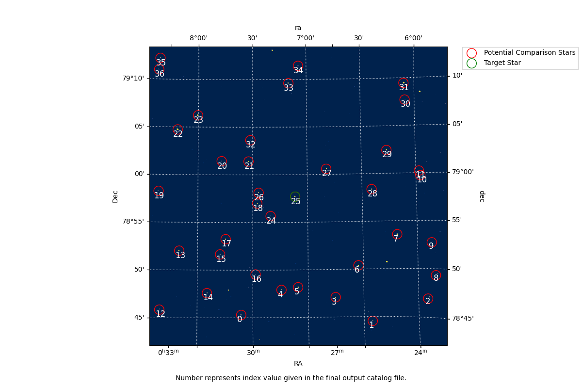
Overlay
An optional overlay plot shows the locations of all comparison stars on a science image, with circles and index numbers marking each star:
def overlay(df, tar_ra, tar_dec, fits_file):
    """
    Creates an overlay of a science image with APASS objects numbered as seen in the catalog file that
    was saved previously

    :param tar_dec: target declination
    :param tar_ra: target right ascension
    :param df: input catalog DataFrame
    :return: None but displays a science image with over-layed APASS objects
    """
    # NSVS_254037-S001-R004-C001-Empty-R-B2.fts
    # fits_file = input("Enter file pathway to one of your science image files for creating an overlay or "
    #                   "comparison stars: ")

    # get the image data for plotting purposes
    header_data_unit_list = fits.open(fits_file)
    image = header_data_unit_list[0].data
    header = header_data_unit_list[0].header

    # set variables to lists
    index_num = list(df[0])
    ra_catalog = list(df[1])
    dec_catalog = list(df[2])

    # convert the lists to degrees for plotting purposes
    ra_cat_new = (np.array(splitter(ra_catalog)) * 15) * u.deg
    dec_cat_new = np.array(splitter(dec_catalog)) * u.deg

    # text for the caption below the graph
    txt = "Number represents index value given in the final output catalog file."

    # Calculate the zscale interval for the image
    zscale = ZScaleInterval()

    # Calculate vmin and vmax for the image display
    vmin, vmax = zscale.get_limits(image)

    # plot the image and the overlays
    wcs = WCS(header)
    fig = plt.figure(figsize=(12, 8))
    fig.text(.5, 0.02, txt, ha='center')
    ax = plt.subplot(projection=wcs)
    plt.imshow(image, origin='lower', cmap='cividis', aspect='equal', vmin=vmin, vmax=vmax)
    plt.xlabel('RA')
    plt.ylabel('Dec')

    overlay = ax.get_coords_overlay('icrs')
    overlay.grid(color='white', ls='dotted')

    ax.scatter(ra_cat_new, dec_cat_new, transform=ax.get_transform('fk5'), s=200,
               edgecolor='red', facecolor='none', label="Potential Comparison Stars")
    ax.scatter((tar_ra * 15) * u.deg, tar_dec * u.deg, transform=ax.get_transform('fk5'), s=200,
               edgecolor='green', facecolor='none', label="Target Star")

    count = 0
    # annotates onto the image the index number and Johnson V magnitude
    for x, y in zip(ra_cat_new, dec_cat_new):
        px, py = wcs.wcs_world2pix(x, y, 0.)
        plt.annotate(str(index_num[count]), xy=(px + 30, py - 50), color="white", fontsize=12)
        count += 1

    plt.gca().invert_xaxis()
    plt.legend(bbox_to_anchor=(1.45, 1.01), fancybox=False, shadow=False)
    plt.show()
BSUO or SARA/TESS Night Filters
When using Astro ImageJ (AIJ), it produces .dat files containing magnitude and
flux data for each night of observations. This program combines all nightly files
into a single file per filter.
The program checks whether the .dat files contain five columns (magnitude only)
or seven columns (magnitude and flux) and writes the combined output accordingly:
2458379.568521	11.151862	0.00268
2458379.57057	11.156097	0.002681
2458379.574054	11.154805999999999	0.003379
2458379.575709	11.171213999999999	0.003407
2458379.577341	11.175478	0.0034130000000000002
2458379.578996	11.18955	0.0034289999999999998
2458379.5806279997	11.193944	0.0034170000000000003
2458379.58226	11.204361	0.00344
2458379.583904	11.207133	0.0034270000000000004
2458379.585524	11.217825	0.003436
2458379.587156	11.242205	0.003474
2458379.588812	11.23937	0.00346
2458379.590444	11.2604	0.0034770000000000005
2458379.592076	11.271894	0.0035020000000000003
2458379.593708	11.282343	0.003532
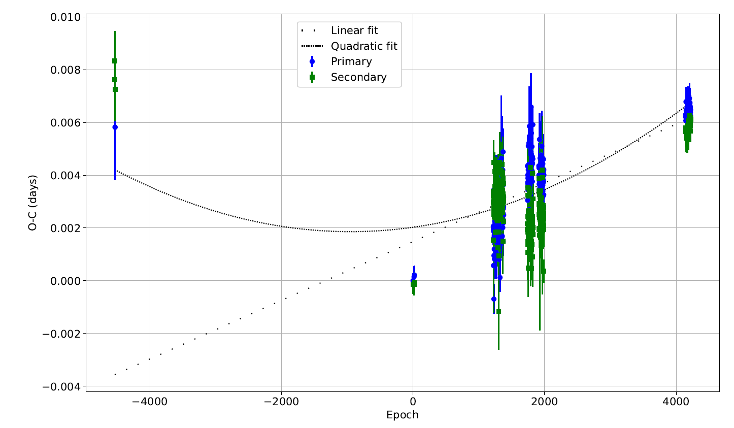
O-C Plotting
The O-C plotting panel calculates Observed minus Calculated (O-C) values given a period and times of minimum (ToM), then fits linear and quadratic models to the data.
The GUI panel offers three modes selected by radio buttons:
BSUO/SARA — averages ToM across Johnson B, V, and Cousins R filters
TESS — processes a single TESS ToM file
All Data — merges multiple pre-calculated O-C files into one combined dataset
Common inputs across all modes:
Period — orbital period of the system in days
Output Folder — where all output files will be saved
I already have an Epoch value — checkbox to enter a known T0 and its error; if unchecked the first ToM in the data is used as T0
BSUO/SARA
Requires three ToM files, one per filter (B, V, R). The program averages the three filters for each epoch:
def BSUO(T0, To_err, period, db, dv, dr):
    """
    This function uses BSUO filter ToM's to calculate and averaged ToM from the 3 filters used. Then calculates
    O-C values to be plotted later.

    :return: output file that will be used to plot the O-C data
    """
    # strict Kwee van Woerden method ToM for all 3 filters
    strict_B = list(db[0])
    strict_B_err = list(db[2])
    strict_V = list(dv[0])
    strict_V_err = list(dv[2])
    strict_R = list(dr[0])
    strict_R_err = list(dr[2])

    # create the lists that will be used
    E_est = []
    O_C = []
    O_C_err = []
    average_min = []
    average_err = []

    # calculates the minimum by averaging the three filters together and getting the total error for that averaged ToM
    for count, val in enumerate(strict_B):
        # calculate ToM and its error
        minimum = (val + strict_V[count] + strict_R[count]) / 3
        err = sqrt(strict_B_err[count] ** 2 + strict_V_err[count] ** 2 + strict_R_err[count] ** 2) / 3

        average_min.append("%.5f" % minimum)
        average_err.append(err)

        # call the function to calculate the O-C values
        e, OC, OC_err, T0, To_err = calculate_oc(minimum, err, T0, To_err, period)
        E_est.append(e)
        O_C.append(OC)
        O_C_err.append(OC_err)

    # create a dataframe for all outputs to be places in for easy output
    dp = pd.DataFrame({
        "Minimums": average_min,
        "Epoch": E_est,
        "O-C": O_C,
        "O-C_Error": O_C_err
    })

    # output file name to place the above dataframe into for saving
    outfile = input("Please enter the output fil pathway and file name with extension for the ToM "
                    "(i.e. C:\\folder1\\test.txt): ")
    # noinspection PyTypeChecker
    dp.to_csv(outfile, index=None, sep="\t")
    print("\nFinished saving file to " + outfile + ". This file is in the same folder as this python program.")

    return outfile
TESS
Requires a single ToM file. No averaging is performed as only one filter is available:
def TESS_OC(T0, To_err, period, df):
    """
    This function takes ToM data pre-gathered from TESS data and finds corresponding O-C values.

    :return: output file that will be used to plot the O-C data
    """
    # strict Kwee van Woerden method ToM
    min_strict = list(df[0])
    min_strict_err = list(df[2])

    # modified Kwee van Woerdan method ToM for potential use later
    # min_mod = list(df[3])
    # min_mod_err = list(df[4])

    # create the lists that will be used
    E_est = []
    O_C = []
    O_C_err = []

    # this for loop, loops through the min_strict list and calculates a variety of values
    for count, val in enumerate(min_strict):
        # call the function to calculate the O-C values
        e, OC, OC_err, T0, To_err = calculate_oc(val, min_strict_err[count], T0, To_err, period)

        E_est.append(e)
        O_C.append(OC)
        O_C_err.append(OC_err)

    # create a dataframe for all outputs to be places in for easy output
    dp = pd.DataFrame({
        "Minimums": min_strict,
        "Epoch": E_est,
        "O-C": O_C,
        "O-C_Error": O_C_err
    })

    # output file name to place the above dataframe into for saving
    outfile = input("Please enter the output file pathway and file name with extension for the ToM "
                    "(i.e. C:\\folder1\\test.txt): ")
    dp.to_csv(outfile, index=None, sep="\t")
    print("\nFinished saving file to " + outfile + ". This file is in the same folder as this python program.")

    return outfile
All Data
Note
All input files must follow the format shown in example_OC_table.txt.
Accepts a comma-separated list of pre-calculated O-C files and merges them into a single output. A LaTeX-formatted table is also produced automatically:
def all_data(nights, period, loop):
    """
    Merges all the data into a singular file for ease of use

    :param nights: number of files there are for the first time through
    :param period: period of the system
    :param loop: number of loops through the program either o or 1

    :return: None
    """
    count = 0

    minimum_list = []
    e_list = []
    o_c_list = []
    o_c_err_list = []

    while True:
        print("\n\nPlease make sure that the very first line for each and every file that you have starts with the following\n"
              "'Minimums	Epoch	O-C	O-C_Error'\n"
              "With each space entered as a space.\n")
        fname = input("Please enter a file name and pathway (i.e. C:\\folder1\\folder2\\[file name]): ")
        df = pd.read_csv(fname, header=None, skiprows=[0], delim_whitespace=True)
        minimum = np.array(df[0])
        e = np.array(df[1])
        o_c = np.array(df[2])
        o_c_err = np.array(df[3])

        for num, val in enumerate(minimum):
            minimum_list.append("%.5f" % val)
            e_list.append(e[num])
            o_c_list.append("%.5f" % o_c[num])
            o_c_err_list.append("%.5f" % o_c_err[num])
        if count + 1 == nights:
            break
        else:
            count += 1
            continue
    dp = pd.DataFrame({
        "Minimums": minimum_list,
        "Epoch": e_list,
        "O-C": o_c_list,
        "O-C_Error": o_c_err_list
    })

    outfile = input("Please enter the output file pathway and file name WITHOUT extension "
                    "for the ToM (i.e. C:\\folder\[file_name]): ")
    dp.to_csv(outfile + ".txt", index=None, sep="\t")
    print("\nFinished saving file to " + outfile + ".txt\n")

    # LaTeX table stuff, don't change unless you know what you're doing!

    table_header = "\\renewcommand{\\baselinestretch}{1.00} \small\\normalsize"
    table_header += '\\begin{center}\n' + '\\begin{longtable}{ccc}\n'
    table_header += '$BJD_{\\rm TDB}$ & ' + 'E & ' + 'O-C \\\ \n'
    table_header += '\\hline\n' + '\\endfirsthead\n'
    table_header += '\\multicolumn{3}{c}\n'
    table_header += '{\\tablename\ \\thetable\ -- \\textit{Continued from previous page}} \\\ \n'
    table_header += '$BJD_{\\rm TDB}$ & E & O-C \\\ \n'
    table_header += '\\hline\n' + '\\endhead\n' + '\\hline\n'
    table_header += '\\multicolumn{3}{c}{\\textit{Continued on next page}} \\\ \n'
    table_header += '\\endfoot\n' + '\\endlastfoot\n'

    minimum_lines = []
    for i in range(len(minimum)):
        line = str("%.5f" % minimum[i]) + ' & ' + str(e[i]) + ' & $' + str("%.5f" % o_c[i]) + ' \pm ' + str(
            "%.5f" % o_c_err[i]) + '$ ' + "\\\ \n"
        minimum_lines.append(line)

    output = table_header
    for count, line in enumerate(minimum_lines):
        output += line

    output += '\\hline\n' + '\\caption{NSVS 896797 O-C. The first column is the \n' \
                            '$BJD_{TDB}$ and column 2 is the epoch number with a whole number \n' \
                            'being a primary eclipse and a half integer value being a secondary \n' \
                            'eclipse. Column 3 is the $(O-C)$ value with the corresponding \n' \
                            '1$\\sigma$ error.}\n' \
              + '\\label{tbl:896797_OC}\n' + '\\end{longtable}\n' + '\\end{center}\n'
    output += '\\renewcommand{\\baselinestretch}{1.66} \\small\\normalsize'
    """
    End LaTeX table stuff.
    """

    # outputfile = input("Please enter an output file name without the extension: ")
    file = open(outfile + ".tex", "w")
    file.write(output)
    file.close()

    outfile += ".txt"

    data_fit(outfile, period, loop, nights)
\renewcommand{\baselinestretch}{1.00} \small\normalsize\begin{center}
\begin{longtable}{ccc}
$BJD_{\rm TDB}$ & E & O-C \\
\hline
\endfirsthead
\multicolumn{3}{c}
{\tablename\ \thetable\ -- \textit{Continued from previous page}} \\
$BJD_{\rm TDB}$ & E & O-C \\
\hline
\endhead
\hline
\multicolumn{3}{c}{\textit{Continued on next page}} \\
\endfoot
\endlastfoot
2457143.76135 & 0.0 & $-0.00001 \pm 0.00020$ \\
2457143.91771 & 0.5 & $-0.00014 \pm 0.00026$ \\
2457161.75645 & 57.5 & $-0.00051 \pm 0.00020$ \\
2457161.91298 & 58.0 & $-0.00046 \pm 0.00019$ \\
\hline
\caption{NSVS 896797 O-C. The first column is the
$BJD_{TDB}$ and column 2 is the epoch number with a whole number
being a primary eclipse and a half integer value being a secondary
eclipse. Column 3 is the $(O-C)$ value with the corresponding
1$\sigma$ error.}
\label{tbl:896797_OC}
\end{longtable}
\end{center}
\renewcommand{\baselinestretch}{1.66} \small\normalsize
Calculations
The core O-C calculation is handled by the calculate_oc function:
@jit(forceobj=True)
def calculate_oc(m, err, T0, T0_err, p):
    """
    Calculates O-C values and errors and find the eclipse number for primary and secondary eclipses
    :param m: ToM
    :param err: ToM error
    :param T0: first ToM
    :param T0_err: error for the T0
    :param p: period of the system

    :return: e (eclipse number), OC (O-C value), OC_err (corresponding O-C error)
    """
    if T0 == 0:
        T0 = m
        T0_err = err
    # get the exact E value
    E_act = (m - T0) / p
    # estimate for the primary or secondary eclipse by rounding to the nearest 0.5
    if E_act<=0:
        # if this is floor then the value would round down to a lower value instead of rounding up, results in values being off by 0.5
        e=ceil((E_act*2)+0.5)/2
    else:
        e=floor((E_act*2)+0.5)/2

    # calculate the calculated ToM and find the O-C value
    T_calc = T0 + (e * p)
    OC = "%.5f" % (m - T_calc)

    # determine the error of the O-C
    OC_err = "%.5f" % sqrt(T0_err ** 2 + err ** 2)

    return e, OC, OC_err, T0, T0_err
The Numba @jit decorator accelerates this function.
The eclipse number is determined using floor (positive epoch) or ceiling (negative epoch),
and O-C values are rounded to five decimal places.
Minimums	Eclipse_#	O-C	O-C_Error
2457143.76182	0.0	0.00000	0.00014
2457143.91854	0.5	-0.00008	0.00028
2457161.75726	57.5	-0.00088	0.00022
2457161.91375	58.0	-0.00088	0.00019
2458842.68058	5428.5	-0.03889	0.00051
2458842.83709	5429.0	-0.03885	0.00083
2458842.99348	5429.5	-0.03895	0.00050
2458843.14992	5430.0	-0.03900	0.00096
2458843.30633	5430.5	-0.03907	0.00046
Fitting and Output
After calculating O-C values, data_fit performs both a linear and quadratic weighted
least squares fit. Output files written to the output folder:
[mode]_OC.txt— the O-C data table[mode]_OC.png— the O-C plot with linear and quadratic fits[mode]_OC.tex— regression tables formatted for LaTeX
def data_fit(input_file, period, loop, nights):
    """
    Create a linear fit by hand and then use scipy to create a polynomial fit given an equation along with their
    respective residual plots

    :param nights: number of files the user has
    :param loop: number of loops the program has gone through either 0 or 1
    :param period: period of the system
    :param input_file: input file from either TESS or BSUO

    :return: None
    """
    # read in the text file
    df = pd.read_csv(input_file, header=0, delim_whitespace=True)

    # append values to their respective lists for further and future potential use
    x = df["Epoch"]
    y = df["O-C"]
    y_err = df["O-C_Error"]

    # weights for least squares fitting
    weights = 1 / (y_err ** 2)

    # these next parts are mainly for O-C data as I just want to plot primary minima's and not both primary/secondary
    x1_prim = []
    y1_prim = []
    y_err_new_prim = []

    x1_sec = []
    y1_sec = []
    y_err_new_sec = []

    # collects primary and secondary times of minima separately and its corresponding O-C and O-C error
    for count, val in enumerate(x):
        # noinspection PyUnresolvedReferences
        if val % 1 == 0:  # checks to see if the eclipse number is primary or secondary
            x1_prim.append(float(val))
            y1_prim.append(float(y[count]))
            y_err_new_prim.append(float(y_err[count]))
        else:
            x1_sec.append(float(val))
            y1_sec.append(float(y[count]))
            y_err_new_sec.append(float(y_err[count]))

    # converts the lists to numpy arrays
    x1_prim = np.array(x1_prim)
    y1_prim = np.array(y1_prim)
    y_err_new_prim = np.array(y_err_new_prim)

    x1_sec = np.array(x1_sec)
    y1_sec = np.array(y1_sec)
    y_err_new_sec = np.array(y_err_new_sec)

    # different line styles that can be used
    line_style = [(0, (1, 10)), (0, (1, 1)), (0, (5, 10)), (0, (5, 5)), (0, (5, 1)),
                  (0, (3, 10, 1, 10)), (0, (3, 5, 1, 5)), (0, (3, 1, 1, 1)), (0, (3, 5, 1, 5, 1, 5)),
                  (0, (3, 10, 1, 10, 1, 10)), (0, (3, 1, 1, 1, 1, 1))]
    line_count = 0
    i_string = ""

    # beginning latex to a latex table
    beginningtex = """\\documentclass{report}
            \\usepackage{booktabs}
            \\begin{document}"""
    endtex = "\end{document}"

    # opens a file with this name to begin writing to the file
    output_test = None
    while not output_test:
        output_file = input("\nWhat is the output file name and pathway for the regression tables (either .txt or .tex): ")
        if output_file.endswith((".txt", ".tex")):
            output_test = True
        else:
            print("This is not an allowed file output. Please make sure the file has the extension .txt or .tex.\n")

    # noinspection PyUnboundLocalVariable
    f = open(output_file, 'w')
    f.write(beginningtex)

    # sets up the fitting parameters
    xs = np.linspace(x.min(), x.max(), 1000)
    degree = 2
    degree_list = ["Linear", "Quadratic"]
    # noinspection PyUnboundLocalVariable
    for i in range(1, degree + 1):
        """
        Inside the model variable:
        'np.polynomial.polynomial.polyfit(x, y, i)' gathers the coefficients of the line fit

        'Polynomial' then finds an array of y values given a set of x data
        """
        model = Polynomial(np.polynomial.polynomial.polyfit(x1_prim, y1_prim, i))

        # plot the main graph with both fits (linear and poly) onto the same graph
        plt.plot(xs, model(xs), color="black", label=degree_list[i - 1] + " fit",
                 linestyle=line_style[line_count])
        line_count += 1

        # this if statement adds a string together to be used in the regression analysis
        # pretty much however many degrees in the polynomial there are, there will be that many I values
        if i >= 2:
            i_string = i_string + " + I(x**" + str(i) + ")"
            mod = smf.wls(formula='y ~ x' + i_string, data=df, weights=weights)
            res = mod.fit()
            f.write(res.summary().as_latex())
        elif i == 1:
            mod = smf.wls(formula='y ~ x', data=df, weights=weights)
            res = mod.fit()
            if loop == 0:
                period_add = res.params[1]
                new_period = period + period_add
                print("The amount added to the period to get the adjusted period is " + str(period_add) + " days.")
                print("The new period then becomes " + str(new_period) + " days.")
            f.write(res.summary().as_latex())

    f.write(endtex)
    # writes to the file the end latex code and then saves the file
    f.close()
    print("\nFinished saving latex/text file.\n\n")

    fontsize = 14
    plt.errorbar(x1_prim, y1_prim, yerr=y_err_new_prim, fmt="o", color="blue", label="Primary")
    plt.errorbar(x1_sec, y1_sec, yerr=y_err_new_sec, fmt="s", color="green", label="Secondary")
    # allows the legend to be moved wherever the user wants the legend to be placed rather than in a fixed location
    print("\n\n\033[1m" + "\033[93m" + "NOTE" + "\033[00m" + ":")
    print("You can drag the legend to move it wherever you would like, the default is the top right. Just click and drag"
          " to move around the figure.\n")
    plt.legend(loc="upper right", fontsize=fontsize).set_draggable(True)

    x_label = "Epoch"
    y_label = "O-C (days)"

    if loop == 0:
        print("\nThe figure just plotted is with the original period. The program will start over using a "
              "new period based on the linear fit.\n")

    # noinspection PyUnboundLocalVariable
    plt.xlabel(x_label, fontsize=fontsize)
    plt.xticks(fontsize=fontsize)
    # noinspection PyUnboundLocalVariable
    plt.ylabel(y_label, fontsize=fontsize)
    plt.yticks(fontsize=fontsize)
    plt.grid()
    time.sleep(1)
    plt.show()

    if loop == 0:
        loop += 1
        main(new_period, loop, nights)
\documentclass{report}
            \usepackage{booktabs}
            \begin{document}\begin{center}
\begin{tabular}{lclc}
\toprule
\textbf{Dep. Variable:}    &        y         & \textbf{  R-squared:         } &     0.982   \\
\textbf{Model:}            &       OLS        & \textbf{  Adj. R-squared:    } &     0.982   \\
\textbf{Method:}           &  Least Squares   & \textbf{  F-statistic:       } & 4.945e+04   \\
\textbf{Date:}             & Tue, 28 Mar 2023 & \textbf{  Prob (F-statistic):} &     0.00    \\
\textbf{Time:}             &     19:10:00     & \textbf{  Log-Likelihood:    } &    5410.8   \\
\textbf{No. Observations:} &         903      & \textbf{  AIC:               } & -1.082e+04  \\
\textbf{Df Residuals:}     &         901      & \textbf{  BIC:               } & -1.081e+04  \\
\textbf{Df Model:}         &           1      & \textbf{                     } &             \\
\textbf{Covariance Type:}  &    nonrobust     & \textbf{                     } &             \\
\bottomrule
\end{tabular}
\begin{tabular}{lcccccc}
                   & \textbf{coef} & \textbf{std err} & \textbf{t} & \textbf{P$> |$t$|$} & \textbf{[0.025} & \textbf{0.975]}  \\
\midrule
\textbf{Intercept} &       0.0001  &        0.000     &     0.895  &         0.371        &       -0.000    &        0.000     \\
\textbf{x}         &   -3.991e-06  &     1.79e-08     &  -222.382  &         0.000        &    -4.03e-06    &    -3.96e-06     \\
\bottomrule
\end{tabular}
\begin{tabular}{lclc}
\textbf{Omnibus:}       & 96.524 & \textbf{  Durbin-Watson:     } &     1.917  \\
\textbf{Prob(Omnibus):} &  0.000 & \textbf{  Jarque-Bera (JB):  } &   482.165  \\
\textbf{Skew:}          & -0.342 & \textbf{  Prob(JB):          } & 1.99e-105  \\
\textbf{Kurtosis:}      &  6.514 & \textbf{  Cond. No.          } &  4.27e+04  \\
\bottomrule
\end{tabular}
%\caption{OLS Regression Results}
\end{center}
Gaia Search
Query
Some Gaia functionality is described in the AIJ Comparison Star Selector section. The Gaia Search panel queries Gaia DR3 for physical parameters of a target star.
The GUI panel accepts the following inputs:
Right Ascension (RA) — format
HH:MM:SS.SSSSDeclination (DEC) — format
DD:MM:SS.SSSSor-DD:MM:SS.SSSSOutput File Path — folder where the results CSV will be saved
The query returns the top four matches within a 5 arcsecond search cone and saves the following parameters:
Parallax and error
Distance (lower, central, upper)
Effective temperature (lower, central, upper)
Gaia G, BP, and RP magnitudes
Radial velocity and error
def target_star(ra_input, dec_input, output_path, write_callback=None, cancel_event=None):
    """
    This queries Gaia DR3 all the parameters below, but I only outputted the specific parameters that are (at the moment)
    the most important for current research at BSU

    :return: Outputs a file with the specific parameters
    """

    def log(message):
        """Log messages to the GUI if callback provided, otherwise print"""
        if write_callback:
            write_callback(message)
        else:
            print(message)

    try:
        if cancel_event.is_set():
            log("Task canceled.")
            return

        ra_input2 = splitter([ra_input])
        dec_input2 = splitter([dec_input])

        ra = ra_input2[0] * 15
        dec = dec_input2[0]

        g = GaiaData.from_query("""
        SELECT TOP 2000
        gaia_source.source_id,gaia_source.ra,gaia_source.dec,gaia_source.parallax,gaia_source.parallax_error,
        gaia_source.pmra,gaia_source.pmdec,gaia_source.ruwe,gaia_source.phot_g_mean_mag,gaia_source.bp_rp,
        gaia_source.radial_velocity,gaia_source.radial_velocity_error,gaia_source.rv_method_used,
        gaia_source.phot_variable_flag,gaia_source.non_single_star,gaia_source.has_xp_continuous,
        gaia_source.has_xp_sampled,gaia_source.has_rvs,gaia_source.has_epoch_photometry,gaia_source.has_epoch_rv,
        gaia_source.has_mcmc_gspphot,gaia_source.has_mcmc_msc,gaia_source.teff_gspphot,gaia_source.teff_gspphot_lower,
        gaia_source.teff_gspphot_upper,gaia_source.logg_gspphot,
        gaia_source.mh_gspphot,gaia_source.distance_gspphot,gaia_source.distance_gspphot_lower,
        gaia_source.distance_gspphot_upper,gaia_source.azero_gspphot,gaia_source.ag_gspphot,
        gaia_source.ebpminrp_gspphot,gaia_source.phot_g_mean_mag,gaia_source.phot_bp_mean_mag,gaia_source.phot_rp_mean_mag
        FROM gaiadr3.gaia_source
        WHERE
        CONTAINS(
            POINT('ICRS',gaiadr3.gaia_source.ra,gaiadr3.gaia_source.dec),
            CIRCLE(
                'ICRS',
                COORD1(EPOCH_PROP_POS({}, {},4.7516,48.8840,-24.1470,0,2000,2016.0)),
                COORD2(EPOCH_PROP_POS({}, {},4.7516,48.8840,-24.1470,0,2000,2016.0)),
                0.001388888888888889)
        )=1""".format(ra, dec, ra, dec))

        if cancel_event.is_set():
            log("Task canceled.")
            return

        # to add parameters to the output file, add them here and the format for the parameter is 'g.[param name from above]'
        df = pd.DataFrame({
            "Parallax(mas)": g.parallax[:4],
            "Parallax_err(mas)": g.parallax_error[:4],
            "Distance_lower(pc)": g.distance_gspphot_lower[:4],
            "Distance(pc)": g.distance_gspphot[:4],
            "Distance_higher(pc)": g.distance_gspphot[:4],
            "T_eff_lower(K)": g.teff_gspphot_lower[:4],
            "T_eff(K)": g.teff_gspphot[:4],
            "T_eff_higher(K)": g.teff_gspphot_upper[:4],
            "G_Mag": g.phot_g_mean_mag[:4],
            "G_BP_Mag": g.phot_bp_mean_mag[:4],
            "G_RP_Mag": g.phot_rp_mean_mag[:4],
            "Radial_velocity(km/s)": g.radial_velocity[:4],
            "Radial_velocity_err(km/s)": g.radial_velocity_error[:4],
        })

        output_file = os.path.join(output_path, "gaia_results.csv")

        df.to_csv(output_file, sep="\t")

        log("\n For more information on each of the output parameters please reference this webpage: "
              "https://gea.esac.esa.int/archive/documentation/GDR3/Gaia_archive/chap_datamodel/sec_dm_main_source_catalogue/ssec_dm_gaia_source.html")
        log("If any of the parameters have values of '1e+20', then Gaia does not have data on that specific parameter.")

        log("\nFinished Gaia search.\n")
    except Exception as e:
        log(f"An error occurred: {e}")
        raise
Parallax(mas)	Parallax_err(mas)	Distance_lower(pc)	Distance(pc)	Distance_higher(pc)	T_eff_lower(K)	T_eff(K)	T_eff_higher(K)	G_Mag	G_BP_Mag	G_RP_Mag	Radial_velocity(km/s)	Radial_velocity_err(km/s)
4.751641342780107	0.011979661	1e+20	1e+20	1e+20	1e+20	1e+20	1e+20	11.719252	12.113523	11.06324	-42.200104	24.182922
Note
Parameters with a value of 1e+20 indicate that Gaia does not have data for
that parameter for the given star. Full parameter descriptions are available at the
Gaia archive documentation.
O’Connell Effect
Note
Based on this paper and originally created by Alec J. Neal.
The GUI panel accepts the following inputs:
Number of Filters — radio buttons to select 1, 2, or 3 filters
File Path(s) — one file per selected filter (Johnson B, V, Cousins R)
HJD — reference epoch (first primary ToM)
Period — orbital period in days
System Name — used for output file naming
Output File Path — folder where results will be saved
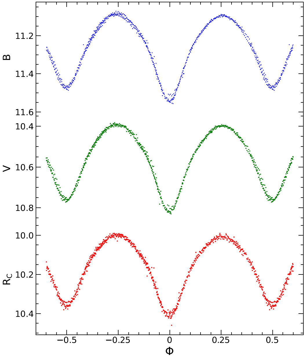
Calculations
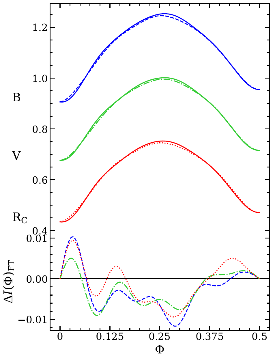
Magnitude data is converted to flux and phased using the period. The first and second halves of the phased light curve are then compared:
def Half_Comp(filter_files, Epoch, period,
              FT_order=10, sections=4, section_order=8,
              resolution=512, offset=0.25, save=False, outName='noname_halfcomp.png',
              title=None, filter_names=None, sans_font=False,
              write_callback=None, cancel_event=None):
    def log(message):
        """Log messages to the GUI if callback provided, otherwise print"""
        if write_callback:
            write_callback(message)
        else:
            print(message)

    if cancel_event.is_set():
        log("Task canceled.")
        return

    # Setting font family if not using sans font
    if sans_font == False:
        plt.rcParams['font.family'] = 'serif'  # Set font family to serif if sans_font is False
        plt.rcParams['mathtext.fontset'] = 'dejavuserif'  # Set math font to serif if sans_font is False

    # Calculate the number of bands
    bands = len(filter_files)

    # Create subplots for flux and dI
    axs, _ = plot.multiplot(figsize=(6, 9), dpi=512, height_ratios=[7 / 3 * bands, 3])
    flux = axs[0]  # Flux subplot
    dI = axs[1]  # dI subplot

    colors = ['blue', 'limegreen', 'red', 'm']  # Color list for plots
    styles = ['--', '-.', ':', '--']  # Line styles for plots

    R2_halves = []  # List to store R^2 values for each band

    # Draw horizontal line at y=0 on dI subplot
    dI.axhline(0, linestyle='-', color='black', linewidth=1)

    # Loop over each band
    for band in range(bands):
        # Binning of data
        a, b = binning.polybinner(filter_files[band], Epoch, period, sections=sections,
                                  norm_factor='alt', section_order=section_order)[0][:2:]

        half = int(0.5 * resolution) + 1  # Calculate half index for resolution

        # Compute Fourier Transform for positive and negative bins
        FT1 = FT.FT_plotlist(a, b, FT_order, resolution)
        FT2 = FT.FT_plotlist(a, -1 * b, FT_order, resolution)
        FTphase1, FTflux1 = FT1[0][:half:], FT1[1][:half:]  # Positive phase and flux
        FTphase2, FTflux2 = FT2[0][:half:], FT2[1][:half:]  # Negative phase and flux

        # Calculate coefficient of determination (R^2) between positive and negative fluxes
        R2_halves.append(calc.error.CoD(FTflux1, FTflux2))
        R2_halves.append(calc.error.CoD(FTflux2, FTflux1))

        dIlist = []  # List to store dI values
        for phase in FTphase1:
            dIlist.append(dI_phi(b, phase, FT_order))  # Calculate dI values

        # Adjust flux values for plotting
        FTflux1 = np.array(FTflux1) + (1 - band) * offset
        FTflux2 = np.array(FTflux2) + (1 - band) * offset

        # Plot flux and dI
        flux.plot(FTphase1, FTflux1, linestyle=styles[band], color=colors[band])
        flux.plot(FTphase2, FTflux2, '-', color=colors[band])

        # Add filter names to flux subplot if provided
        if filter_names is not None:
            if len(filter_names) == bands:
                flux.text(-0.12, FTflux1[0], filter_names[band], fontsize=18, rotation=0)

        # Plot dI
        dI.plot(FTphase1, dIlist, linestyle=styles[band], color=colors[band])

    if cancel_event.is_set():
        log("Task canceled.")
        return

    # Set x-axis limit for flux subplot
    plt.xlim(-0.025, 0.525)

    # Set y-axis label for flux subplot if filter_names is None
    if filter_names is None:
        flux.set_ylabel('Flux', fontsize=16)

    # Format subplots
    plot.sm_format(flux, numbersize=15, X=0.125, x=0.025, xbottom=False, bottomspine=False, Y=None)
    plot.sm_format(dI, numbersize=15, X=0.125, x=0.025, xtop=False, topspine=False)
    dI.set_xlabel(r'$\Phi$', fontsize=18)  # Set x-axis label for dI subplot
    dI.set_ylabel(r'$\Delta I(\Phi)_{\rm FT}$', fontsize=18)  # Set y-axis label for dI subplot

    # Set title for flux subplot if title is not empty
    if title != '':
        flux.set_title(title, fontsize=14.4, loc='left')

    # Save figure if save is True
    if save:
        plt.savefig(outName, bbox_inches='tight')
        log(outName + ' saved.')

    # plt.show()  # Show the plot

    # Reset font settings to default
    plt.rcParams['font.family'] = 'sans'
    plt.rcParams['mathtext.fontset'] = 'dejavusans'

    return None  # Return "Done" message
Statistical values (OER, LCA, ΔI) are calculated for each filter using Monte Carlo simulations (1000 by default):
def OConnell_total(inputFile, Epoch, period, order, sims=1000,
                   sections=4, section_order=8, norm_factor='alt',
                   starName='', filterName='', FT_order=10, FTres=500,
                   write_callback=None, cancel_event=None):
    """
    This function calculates various parameters related to the O'Connell Effect.
    It performs Monte Carlo simulations to estimate errors.
    Approximate runtime: ~ sims/1000 minutes.
    """

    def log(message):
        """Log messages to the GUI if callback provided, otherwise print"""
        if write_callback:
            write_callback(message)
        else:
            print(message)

    if cancel_event.is_set():
        log("Task canceled.")
        return

    """
    Generating master parameters from the observational data.
    """
    # ============================== DO NOT CHANGE ==============================
    # Binning the data
    PB = binning.polybinner(inputFile, Epoch, period, sections=sections, norm_factor=norm_factor,
                            section_order=section_order, FT_order=FT_order)
    c_MB = PB[1][0]  # Correct phase bins and fluxes
    nc_MB = PB[1][1]  # Non-corrected phase bins and fluxes
    ob_phaselist = c_MB[0][1]  # Corrected phase list
    ob_fluxlist = c_MB[1][1]  # Corrected flux list
    ob_fluxerr = c_MB[1][2]  # Corrected flux error list
    c_sec_phases = c_MB[5][0]  # Corrected section phases
    nc_sec_phases = nc_MB[5][0]  # Non-corrected section phases
    c_sec_index = c_MB[5][3]  # Corrected section index
    nc_sec_index = nc_MB[5][3]  # Non-corrected section index

    a = PB[0][0]  # Fourier coefficients (cosine terms)
    b = PB[0][1]  # Fourier coefficients (sine terms)
    # ==========================================================================

    FTsynth = FT.synth(a, b, ob_phaselist, FT_order)  # synthetic FT curve
    master_simflux = []
    for sim in tqdm(range(sims), desc='Simulating light curves', position=0):
        master_simflux.append(FT.sim_ob_flux(FTsynth, ob_fluxerr))
    # ============
    if cancel_event.is_set():
        log("Task canceled.")
        return
    # ============
    c_master_simflux = []
    nc_master_simflux = []
    master_polyflux = []
    """
    List of the resampled polynomial fluxes. Each embedded list is different
    because the generating data has been Monte Carloed.
    """
    master_FTflux = []  # FT fluxes resulting from the simulations
    master_a = []
    master_b = []  # Lists of the a and b FT coefficients for each sim
    OERlist, LCAlist, dIlist, dIavelist = [], [], [], []

    # = begin sim loop =
    for sim in tqdm(range(sims), desc='Simulation processing', position=0):
        """
        Generating empty lists so that stuff can be inserted into the
        specified [sim] index. Otherwise when trying to append list[sim],
        it would throw an error (there'd be nothing to append to).
        """
        c_master_simflux.append([])
        nc_master_simflux.append([])

        # == begin section loop ===
        for section in range(sections):
            c_master_simflux[sim].append([])  # same as before
            nc_master_simflux[sim].append([])

            """
            'Replacing' the observational fluxes with the Monte Carlo fluxes
            based on the index of each data point when it was in ob_fluxlist
            (the MC fluxes are ordered the same as ob_fluxlist).
            """
            for i in range(len(c_sec_phases[section])):
                c_master_simflux[sim][section].append(master_simflux[sim][c_sec_index[section][i]])
            for i in range(len(nc_sec_phases[section])):
                nc_master_simflux[sim][section].append(master_simflux[sim][nc_sec_index[section][i]])
        # == end section loop == ; resume sim loop

        # Generating polynomial resampled fluxes for each simulation.
        minipoly = binning.minipolybinner(c_sec_phases, c_master_simflux[sim],
                                          nc_sec_phases, nc_master_simflux[sim],
                                          section_order)
        master_polyflux.append(minipoly[1])

        # Calculating various parameters for each simulation.
        FTcoef = FT.coefficients(master_polyflux[sim])
        master_a.append(FTcoef[1])
        master_b.append(FTcoef[2])
        master_FTflux.append(FT.FT_plotlist(master_a[sim], master_b[sim], FT_order, FTres)[1])
        OERlist.append(OConnell.OER_FT(master_a[sim], master_b[sim], FT_order))
        LCAlist.append(OConnell.LCA_FT(master_a[sim], master_b[sim], FT_order, 256))
        dIlist.append(OConnell.Delta_I_fixed(master_b[sim], FT_order))
        dIavelist.append(OConnell.Delta_I_mean_obs_noerror(ob_phaselist, ob_fluxlist, phase_range=0.05))
    # = end sim loop =

    if cancel_event.is_set():
        log("Task canceled.")
        return

    # === end Monte Carlo ===

    """
    Calculating FT model errors, as opposed to the errors calculated
    with the simulate light curves.
    """
    a0sig, a0rat = FT.a_sig_fast(a, b, 0, a[0], ob_phaselist, ob_fluxlist, ob_fluxerr, order)
    a_model_err = [a0sig]
    b_model_err = [0]
    a_rat = [a0rat]
    b_rat = [1]
    for n in tqdm(range(1, order + 1), position=0, desc='Calculating FT errors'):
        # TODO, dx0=1 isn't fullproof
        asig, ar = FT.a_sig_fast(a, b, n, a[n], ob_phaselist, ob_fluxlist, ob_fluxerr, order, dx0=1)
        bsig, br = FT.b_sig_fast(a, b, n, b[n], ob_phaselist, ob_fluxlist, ob_fluxerr, order, dx0=1)
        a_model_err.append(asig)
        b_model_err.append(bsig)
        a_rat.append(ar)
        b_rat.append(br)

    if cancel_event.is_set():
        log("Task canceled.")
        return

    # == FT coefficients ==
    a_MC_err = np.array(list(map(st.stdev, zip(*master_a))))
    b_MC_err = np.array(list(map(st.stdev, zip(*master_b))))
    a_total_err = (np.array(a_model_err) ** 2 + a_MC_err[:order + 1:] ** 2) ** 0.5
    b_total_err = (np.array(b_model_err) ** 2 + b_MC_err[:order + 1:] ** 2) ** 0.5

    a2_0125_a2 = a[2] * (0.125 - a[2])
    a2_0125_a2_err = sig_f(lambda x: x * (0.125 - x), a[2], a_total_err[2])

    # == OER ==
    OER = OConnell.OER_FT(a, b, order)
    OER_model_err = OConnell.OER_FT_error_fixed(a, b, a_model_err, b_model_err, order)
    OER_MC_err = st.stdev(OERlist)
    OER_total_err = (OER_model_err ** 2 + OER_MC_err ** 2) ** 0.5

    # == LCA ==
    LCA = OConnell.LCA_FT(a, b, order, 1024)
    LCA_model_err = OConnell.LCA_FT_error(a, b, a_model_err, b_model_err, order, 1024)[1]
    LCA_MC_err = st.stdev(LCAlist)
    LCA_total_err = (LCA_model_err ** 2 + LCA_MC_err ** 2) ** 0.5

    # == Delta_I ==
    Delta_I_025 = OConnell.Delta_I_fixed(b, order)
    Delta_I_025_model_err = OConnell.Delta_I_error_fixed(b_model_err, order)
    Delta_I_025_MC_err = st.stdev(dIlist)
    Delta_I_025_total_err = (Delta_I_025_model_err ** 2 + Delta_I_025_MC_err ** 2) ** 0.5

    # == Delta_I_ave ==
    DIave = OConnell.Delta_I_mean_obs(ob_phaselist, ob_fluxlist, ob_fluxerr, phase_range=0.05, weighted=False)
    Delta_I_ave = DIave[0]
    Delta_I_ave_err = DIave[1]

    # == print parameters ==
    r = lambda x: round(x, 5)

    valerr = lambda x, dx, label, PRECISION=6: print(label + ' =', round(x, PRECISION), '+/-', round(dx, PRECISION))

    # print('\n')
    valerr(a[1], a_total_err[1], 'a1')
    valerr(a[2], a_total_err[2], 'a2')
    valerr(a[4], a_total_err[4], 'a4')
    valerr(a[2] * (0.125 - a[2]),
           sig_f(lambda x: x * (0.125 - x), a[2], (a_model_err[2] ** 2 + a_MC_err[2] ** 2) ** 0.5), 'a2(0.125-a2)')
    # print('')
    valerr(OER, OER_total_err, 'OER')
    # print(r(OER_model_err), r(OER_MC_err), '\n')

    valerr(LCA, LCA_total_err, 'LCA')
    # print(r(LCA_model_err), r(LCA_MC_err), '\n')

    valerr(Delta_I_025, Delta_I_025_total_err, 'Delta_I')
    # print(r(Delta_I_025_model_err), r(Delta_I_025_MC_err), '\n')

    valerr(Delta_I_ave, Delta_I_ave_err, 'Delta_I_ave')

    return [a, a_total_err], [b, b_total_err], [Delta_I_025, Delta_I_025_total_err], [Delta_I_ave, Delta_I_ave_err], [
        OER, OER_total_err], [LCA, LCA_total_err], [a2_0125_a2, a2_0125_a2_err]
See vseq_updated.py for the full mathematical implementations.
Output
A LaTeX-formatted table is produced containing all statistical values for each filter:
def multi_OConnell_total(filter_files, Epoch, period, order=10,
                         sims=1000, sections=4, section_order=8,
                         norm_factor='alt', starName='', filterNames=[r'$\rm B$', r'$\rm V$', r'$\rm R_C$'],
                         FT_order=10, FTres=500, plot_only=False,
                         plotoff=0.25, save=False, outName='noname.png',
                         write_callback=None, cancel_event=None):
    """
    This function generates a half-comparison plot and calculates various parameters related to the O'Connell Effect.
    If plot_only is set to True, only the half-comparison plot will be generated.
    """

    def log(message):
        """Log messages to the GUI if callback provided, otherwise print"""
        if write_callback:
            write_callback(message)
        else:
            print(message)

    if cancel_event.is_set():
        log("Task canceled.")
        return

    # Generate half-comparison plot
    Half_Comp(filter_files, Epoch, period, FT_order=order, sections=sections,
              section_order=section_order, offset=plotoff, save=save, outName=outName,
              filter_names=filterNames, write_callback=write_callback, cancel_event=cancel_event)

    if cancel_event.is_set():
        log("Task canceled.")
        return

    # Perform O'Connell analysis
    if not plot_only:
        filters = len(filter_files)
        a_all = []
        a_err_all = []
        b_all = []
        b_err_all = []
        dI_FT = []
        dI_FT_err = []
        dI_ave = []
        dI_ave_err = []
        OERs = []
        OERs_err = []
        LCAs = []
        LCAs_err = []
        a22s = []
        a22s_err = []

        # Running the O'Connell function on each filter
        for band in range(len(filter_files)):
            oc = OConnell_total(filter_files[band], Epoch, period, order, sims=sims,
                                sections=sections, section_order=section_order,
                                norm_factor=norm_factor, FT_order=order, FTres=FTres,
                                filterName='Filter ' + str(band + 1),
                                write_callback=write_callback, cancel_event=cancel_event)
            a_all.append(oc[0][0])
            a_err_all.append(oc[0][1])
            b_all.append(oc[1][0])
            b_err_all.append(oc[1][1])
            dI_FT.append(oc[2][0])
            dI_FT_err.append(oc[2][1])
            dI_ave.append(oc[3][0])
            dI_ave_err.append(oc[3][1])
            OERs.append(oc[4][0])
            OERs_err.append(oc[4][1])
            LCAs.append(oc[5][0])
            LCAs_err.append(oc[5][1])
            a22s.append(oc[6][0])
            a22s_err.append(oc[6][1])

        if cancel_event.is_set():
            log("Task canceled.")
            return

        # LaTeX table creation
        table_header = '\\begin{table}[H]\n' + '\\begin{center}\n' + '\\begin{tabular}{c|'
        for band in range(filters):
            table_header += 'c'
        table_header += '}\n' + '\\hline\\hline\n' + 'Parameter '
        for band in range(filters):
            table_header += '& Filter ' + str(band + 1)
        table_header += '\\\ \n' + '\\hline\n'

        a1_line = '$a_1$ '
        a2_line = '$a_2$ '
        a4_line = '$a_4$ '
        a22_line = '$a_2(0.125-a_2)$ '
        b1_line = '$2b_1$ '
        dIFT_line = '$\Delta I_{\\rm FT}$ '
        dIave_line = '$\Delta I_{\\rm ave}$ '
        OER_line = 'OER '
        LCA_line = 'LCA '

        strr = lambda x, e=5: str(round(x, e))
        for band in range(filters):
            a1_line += '& $' + strr(a_all[band][1]) + '\pm ' + strr(a_err_all[band][1]) + '$ '
            a2_line += '& $' + strr(a_all[band][2]) + '\pm ' + strr(a_err_all[band][2]) + '$ '
            a4_line += '& $' + strr(a_all[band][4]) + '\pm ' + strr(a_err_all[band][4]) + '$ '
            a22_line += '& $' + strr(a22s[band]) + '\pm ' + strr(a22s_err[band]) + '$ '
            b1_line += '& $' + strr(2 * b_all[band][1]) + '\pm ' + strr(2 * b_err_all[band][1]) + '$ '
            dIFT_line += '& $' + strr(dI_FT[band]) + '\pm ' + strr(dI_FT_err[band]) + '$ '
            dIave_line += '& $' + strr(dI_ave[band]) + '\pm ' + strr(dI_ave_err[band]) + '$ '
            OER_line += '& $' + strr(OERs[band]) + '\pm ' + strr(OERs_err[band]) + '$ '
            LCA_line += '& $' + strr(LCAs[band]) + '\pm ' + strr(LCAs_err[band]) + '$ '

        if cancel_event.is_set():
            log("Task canceled.")
            return

        lines = [a1_line, a2_line, a4_line, a22_line, b1_line, dIFT_line, dIave_line, OER_line, LCA_line]
        for count, _ in enumerate(lines):
            lines[count] += '\\\ \n'

        output = table_header
        for _, line in enumerate(lines):
            output += line
        output += '\\hline\n' + '\\end{tabular}\n' + '\\caption{Fourier and O\'Connell stuff (' + str(
            sims) + ' sims)}\n' + '\\label{tbl:OConnell}\n' + '\\end{center}\n' + '\\end{table}\n'
        # End LaTeX table creation

        # print(output)  # Output LaTeX table to console
        # outputfile = input("Please enter an output file name without the extension: ")
        outputfile = outName.rstrip(".pdf")
        file = open(outputfile + ".txt", "w")
        file.write(output)  # Write LaTeX table to file
        file.close()

    return 'nada'
\begin{table}[H]
\begin{center}
\begin{tabular}{c|ccc}
\hline\hline
Parameter & Filter 1& Filter 2& Filter 3\\
\hline
$a_1$ & $-0.01769\pm 0.00029$ & $-0.01497\pm 0.00024$ & $-0.01428\pm 0.0016$ \\
$a_2$ & $-0.14912\pm 0.00064$ & $-0.14238\pm 0.00068$ & $-0.1405\pm 0.00125$ \\
$a_4$ & $-0.02487\pm 0.0003$ & $-0.02372\pm 0.00033$ & $-0.02319\pm 0.00143$ \\
$a_2(0.125-a_2)$ & $-0.04088\pm 0.00027$ & $-0.03807\pm 0.00028$ & $-0.0373\pm 0.00051$ \\
$2b_1$ & $0.00598\pm 0.00046$ & $0.00481\pm 0.00055$ & $0.00356\pm 0.00314$ \\
$\Delta I_{\rm FT}$ & $0.00646\pm 0.00141$ & $0.00462\pm 0.00177$ & $0.00415\pm 0.00784$ \\
$\Delta I_{\rm ave}$ & $0.00911\pm 0.00049$ & $0.00969\pm 0.00047$ & $0.0058\pm 0.00148$ \\
OER & $1.0138\pm 0.00151$ & $1.01268\pm 0.00205$ & $1.00894\pm 0.01198$ \\
LCA & $0.00456\pm 0.00141$ & $0.00351\pm 0.00151$ & $0.00531\pm 0.00458$ \\
\hline
\end{tabular}
\caption{Fourier and O'Connell stuff (1000 sims)}
\label{tbl:OConnell}
\end{center}
\end{table}
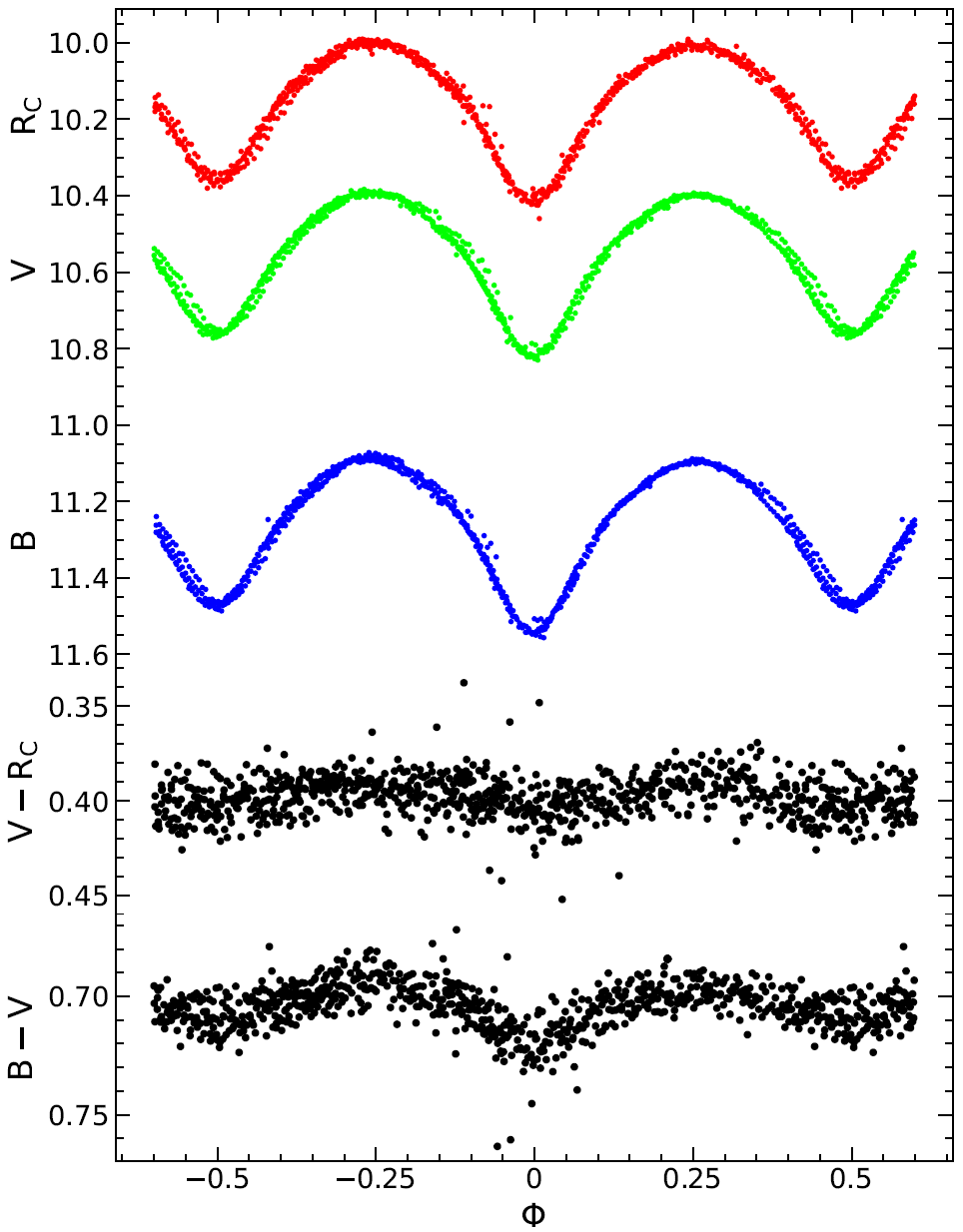
Color Light Curve
Note
Originally created by Alec J. Neal, updated for this package by Kyle Koeller.
The Color Light Curve panel calculates B-V and optionally V-R color indices and effective temperatures from multi-filter light curve data.
The GUI panel accepts the following inputs:
B-band File — Johnson B light curve file
V-band File — Johnson V light curve file
Period — orbital period in days
HJD (Epoch) — first primary ToM
Output Image Name — filename for the saved plot (must end in
.png)
Subtract Light Curve
The subtract_LC function interpolates the B-band observations to the times of
V-band observations, then calculates the instantaneous B-V color index:
def subtract_LC(Bfile, Vfile, Epoch, period,
                max_tol=0.03, lower_lim=0.05, FTinterp=True, quad_range=0.075, index="",
                write_callback=None, cancel_event=None):
    """
    This function actually creates the B-V and R-V values

    :param Bfile: input B file
    :param Vfile: input V file
    :param Epoch: epoch number
    :param period: period of the system
    :param max_tol: maximum tolerance
    :param lower_lim: lower limit
    :param FTinterp: interpolates number
    :param quad_range: ?
    :param index: type of color index to use

    :return: returns the B-V value and other assorted values
    """
    def log(message):
        """Log messages to the GUI if callback provided, otherwise print"""
        if write_callback:
            write_callback(message)
        else:
            print(message)

    B_HJD, B_mag, _ = io.importFile_pd(Bfile)[:3:]
    V_HJD, V_mag, _ = io.importFile_pd(Vfile)[:3:]

    Bpoly = binning.polybinner(Bfile, Epoch, period, sections=2, section_order=8)
    Bphase = Bpoly[1][0][0][1]
    aB = Bpoly[0][0]
    bB = Bpoly[0][1]
    Bnorm = Bpoly[1][0][4]
    Vphase = list(calc.astro.convert.HJD_phase(V_HJD, period, Epoch))
    B_flux = np.array(10 ** (-0.4 * np.array(B_mag))) / Bnorm
    obs = len(V_HJD)
    tolerance = best_tol(B_HJD, V_HJD, period, lower_lim=lower_lim, max_tol=max_tol)
    before_after = occ2(B_HJD, V_HJD, period, tolerance=tolerance)
    befores = before_after[1]
    afters = before_after[2]
    i_before = before_after[3]
    i_after = before_after[4]
    mean_diff = np.mean(before_after[5])

    B_interp_flux = []
    for n in range(obs):
        if len(befores[n]) == 0 or len(afters[n]) == 0:
            B_interp_flux.append(FT.sumatphase(Vphase[n], 10, aB, bB))
        else:
            B_interp_flux.append(lin_interp(V_HJD[n], befores[n][-1], afters[n][0],
                                            B_flux[i_before[n][-1]], B_flux[i_after[n][0]]))

    B_interp_mag = -2.5 * np.log10(np.array(B_interp_flux) * Bnorm)
    # quad_range=0.075
    BVquadphase = []
    BVquadmag = []
    # Vquad=[]
    for n in range(len(Vphase)):
        if 0.25 - quad_range < Vphase[n] < 0.25 + quad_range or 0.75 - quad_range < Vphase[n] < 0.75 + quad_range:
            BVquadphase.append(Vphase[n])
            BVquadmag.append(B_interp_mag[n] - V_mag[n])
    quadcolor = mean_mag(BVquadmag)
    colorerr = st.stdev(BVquadmag, xbar=quadcolor)
    log(str(index) + " " + str(quadcolor) + '+/-' + str(colorerr))

    B_minus_V = B_interp_mag - np.array(V_mag)
    BV_mean = mean_mag(B_minus_V)
    # print(B_minus_V)
    BV_err = st.stdev(B_minus_V, xbar=BV_mean)

    log('ave diff =' + str(round(mean_diff * 100, 3)) + '% of period')
    aVphase, aV_mag, aB_interp_mag = plot.aliasing2(Vphase, V_mag, B_interp_mag)[:3:]
    aBphase, aB_mag = plot.aliasing2(Bphase, B_mag, B_mag)[:2:]
    aB_minus_V = plot.aliasing2(Vphase, B_minus_V, B_minus_V)[1]
    B_V = [B_minus_V, BV_mean, BV_err, aB_minus_V]
    B = [aBphase, aB_mag, aB_interp_mag]
    V = [aVphase, aV_mag]

    # print('T =', vseq.Flower.T.Teff(quadcolor - (0.641 / 3.1)))
    if index == "BV":
        temp = []
        # temp = vseq.Flower.T.Teff(quadcolor - (0.641 / 3.1), colorerr)
        t1 = Flower.T.Teff(quadcolor - (0.641 / 3.1), colorerr)
        temp_high = Flower.T.Teff(quadcolor - (0.641 / 3.1) - colorerr, colorerr)
        temp_low = Flower.T.Teff(quadcolor - (0.641 / 3.1) + colorerr, colorerr)

        # temp_err = (temp_high[0] - temp_low[0])/2
        temp_err = np.sqrt(temp_high[1]**2 + temp_low[1]**2)
        temp.append(t1[0])
        temp.append(temp_err)
        log('T_BV =' + str(temp[0]) + '+/-' + str(temp[1]))
    elif index == "VR":
        t1 = Pecaut.T.Teff(quadcolor - (0.58 / 3.1), colorerr)
        temp = []
        # t1 = Flower.T.Teff(quadcolor - 0.561 * (0.641 / 3.1), colorerr)
        # E_V-R = 0.561*E_B-V
        temp_high = Pecaut.T.Teff(quadcolor - (0.58 / 3.1) - colorerr, colorerr)
        temp_low = Pecaut.T.Teff(quadcolor - (0.58 / 3.1) + colorerr, colorerr)
        # temp_high = Flower.T.Teff(quadcolor - 0.561* (0.641 / 3.1) - colorerr, colorerr)
        # temp_low = Flower.T.Teff(quadcolor - 0.561* (0.641 / 3.1) + colorerr, colorerr)

        # temp_err = (temp_high[0] - temp_low[0]) / 2
        temp_err = np.sqrt(temp_high[1] ** 2 + temp_low[1] ** 2)
        temp.append(t1[0])
        temp.append(temp_err)
        if temp[0] == 0:
            log("V-R color cannot be used to determine temperature.")
        else:
            log('T_VR =' + str(temp[0]) + '+/-' + str(temp[1]))

    return B_V, B, V, quadcolor, colorerr, temp
The effective temperature is derived from the color index using the polynomial fit from Flower 1996 with the Torres 2010 update:
        def Teff(BV, error):
            """
            Calculates the effective temperature (Teff) using the B-V color index.

            Parameters:
                BV (float): B-V color index.
                error (float): Error in B-V color index.

            Returns:
                tuple: A tuple containing the Teff value and its error.
            """
            # Calculate Teff using polynomial approximation
            temp = calc.poly.power(Flower.T.c, BV, 10)
            # Calculate error in Teff using error propagation
            err = calc.poly.t_eff_err(Flower.T.c, BV, error, temp)
            return temp, err
Note
The B-V polynomial is the one Flower specifically derived. Using the same polynomial for V-R is an approximation and should be treated with caution.
Plotting
The output log displays the color index, its error, and the derived effective temperature. The plot shows the phased light curves in the upper panel and the color index variation in the lower panel:
def color_plot(Bfile, Vfile, Epoch, period, max_tol=0.03, lower_lim=0.05, Rfile='', FTinterp=True,
               save=False, outName='noname_color.png', fs=12, write_callback=None, cancel_event=None):
    """
    This is a function version of the GUI and produces the same values but without the plotting aspect

    :param Bfile: input B text file
    :param Vfile: input V text file
    :param Epoch: epoch number
    :param period: period of the system
    :param max_tol: maximum tolerance
    :param lower_lim: lower limit
    :param Rfile: input R text file
    :param FTinterp: interpolate number
    :param save: save the output image
    :param outName: output image name
    :param fs:
    :return: assorted values
    """
    def log(message):
        """Log messages to the GUI if callback provided, otherwise print"""
        if write_callback:
            write_callback(message)
        else:
            print(message)

    B_V = subtract_LC(Bfile, Vfile, Epoch, period, max_tol=max_tol, lower_lim=lower_lim, FTinterp=FTinterp, index="BV", write_callback=write_callback, cancel_event=cancel_event)
    Bphase, Bmag, B_interp_mag = B_V[1][:3:]
    Vphase, Vmag = B_V[2][:2:]
    aB_minus_V = B_V[0][3]
    quadcolor, colorerr = B_V[3:5:]
    if Rfile == '':
        axs, _ = plot.multiplot((7, 7.5), height_ratios=[8, 4.5])
        mag = axs[0]
        bv = axs[1]
        mag.plot(Vphase, Vmag, 'og', ms=2)
        mag.plot(Bphase, Bmag, 'ob', ms=2)
        bv.plot(Vphase, aB_minus_V, 'ok', ms=2)
        bv.margins(y=0.1, x=1 / 24)
        mag.set_ylim(mag.get_ylim()[::-1])
        bv.set_ylim(bv.get_ylim()[::-1])
        plot.sm_format(mag, X=0.25, x=0.05, Y=None, numbersize=fs, xbottom=False, bottomspine=False, tickwidth=1,
                            Xsize=7, xsize=3.5)
        plot.sm_format(bv, X=0.25, x=0.05, numbersize=fs, xtop=False, topspine=False, tickwidth=1, Xsize=7,
                            xsize=3.5)

        maxtick = max(list(map(len, (list(map(str, np.array(mag.get_yticks()).round(8)))))))
        if maxtick == 5:
            ytickpad = -0.835
        else:
            ytickpad = -0.81
        mag.text(ytickpad, (max(Bmag) + min(Bmag)) / 2, 'B', rotation=90, fontsize=fs * 1.2)
        mag.text(ytickpad, (max(Vmag) + min(Vmag)) / 2, 'V', rotation=90, fontsize=fs * 1.2)
        # bv.set_xlabel('$\Phi$',fontsize=fs*1.2)
        bv.set_xlabel('$\Phi$', fontsize=fs * 1.5, usetex=False)
        bv.set_ylabel(r'$\rm B-V$', fontsize=fs * 1.2)
        # quadcolor,colorerr=B_V[3:5:]
        bv.axhline(quadcolor, color='gray', linewidth=None)
    else:
        V_R = subtract_LC(Vfile, Rfile, Epoch, period, max_tol, lower_lim=lower_lim, index="VR")
        Rphase, Rmag = V_R[2][:2:]
        # V_interp_mag = V_R[1][2]
        aV_minus_R = V_R[0][3]
        axs, fig = plot.multiplot((7, 9), height_ratios=[8, 3, 3])
        mag = axs[0]
        bv = axs[2]
        vr = axs[1]
        mag.plot(Vphase, Vmag, 'og', ms=2)
        mag.plot(Bphase, Bmag, 'ob', ms=2)
        mag.plot(Rphase, Rmag, 'or', ms=2)

        bv.plot(Vphase, aB_minus_V, 'ok', ms=3)
        vr.plot(Rphase, aV_minus_R, 'ok', ms=3)
        bv.margins(y=0.07, x=1 / 24)
        vr.margins(y=0.07)
        # mag.margins(y=0.09)
        mag.set_ylim(mag.get_ylim()[::-1])
        bv.set_ylim(bv.get_ylim()[::-1])
        vr.set_ylim(vr.get_ylim()[::-1])
        plot.sm_format(mag, X=0.25, x=0.05, numbersize=fs, xbottom=False, bottomspine=False)
        plot.sm_format(vr, X=0.25, x=0.05, numbersize=fs, xtop=False, topspine=False, xbottom=False,
                            bottomspine=False)
        plot.sm_format(bv, X=0.25, x=0.05, numbersize=fs, xtop=False, topspine=False)
        maxtick = max(list(map(len, (list(map(str, np.array(mag.get_yticks()).round(8)))))))
        if maxtick == 5:
            ytickpad = -0.835
        else:
            ytickpad = -0.81
        mag.text(ytickpad, (max(Bmag) + min(Bmag)) / 2, r'$\rm B$', rotation=90, fontsize=fs * 1.2)
        mag.text(ytickpad, (max(Vmag) + min(Vmag)) / 2, r'$\rm V$', rotation=90, fontsize=fs * 1.2)
        mag.text(ytickpad, (max(Rmag) + min(Rmag)) / 2, r'$\rm R_C$', rotation=90, fontsize=fs * 1.2)
        bv.set_ylabel(r'$\rm B-V$', fontsize=fs * 1.2)
        vr.set_ylabel(r'$\rm V-R_C$', fontsize=fs * 1.2)
        bv.set_xlabel(r'$\Phi$', fontsize=fs * 1.2)
    if save:
        plt.savefig(outName, bbox_inches='tight')
    # plt.show()
    log(f"Color Temp = {quadcolor} {colorerr}")